Heart Disease Prediction Using Neural Networks and Deep Learning

Heart Disease (or Cardiovascular Disease) is a blanket term that generally refers to conditions that involve narrowed or blocked blood vessels. These blockages can then lead to heart attack, angina (chest pain), stroke, or death.
There are several ways to definitively diagnose heart disease, including echocardiograms, MRIs, CT scans, and angiograms. However, these procedures can be expensive for the patient, even if the patient is found to not have heart disease. What if there were a way to screen for heart disease based on a few tests run by a cardiologist?
That’s what this study hoped to achieve:
A screening method that will accurately predict heart disease in a patient based on some simple test results.
To do this, the Cleveland Heart Disease Dataset from UCI was used to train and test both machine learning and deep learning classification models.
Cleaning up the Data
Fortunately, there are only a handful of “useful” data fields in the heart disease dataset, making the ETL job significantly easier than past projects. However, changes still needed to be made and the data scrutinized to make sure that the data was as accurate and clean as possible.
The data was loaded pre-encoded, which is great for analytics and machine learning, but not very intuitive. The documentation provided more insight into the label encoding, and from that, the columns and data could be transformed to something more understandable.
Upon looking at a few datafields, there were several discrepancies that weren’t accounted for in the documentation (for instance, starting variables at 1 instead of 0 for categorical variables). Those were addressed and cleaned up based on the labeled data for greater insight and accuracy during the machine learning phase.
Correlations
There are only 14 variables that are considered “usable” by most studies examining this dataset. However, that doesn’t necessarily mean that we have to use all of them in the machine learning model. Let’s take a look at the correlational heatmap to get a better idea of what to use.

But what if we were to choose only the most important variables?
These are the correlations of the variables from the base dataset. No transformation or scaling has occurred yet, so these are just the raw correlational values. They give a great idea of what to focus on, but we need to know what the absolute best features to use are, and that’s when we use a Chi2 test. The Chi2 test allows us to use categorical variables as well as numerical, whereas the correlational heatmap does not.

So, those are the top 10 best features and the ones that were used in the machine learning models.
Scaling and Encoding
The most tedious process in any machine learning project is data preprocessing and preparation. The data must be scaled and encoded for optimal performance in a machine learning model, as a model can’t determine the value of “United States” or, in this case, “Exercise Induced Angina: Yes/No”. Thankfully, the data was already LabelEncoded, but that only gave numerical values and not something that could make the categorical variables directly comparable to each other for use in categorization.
To begin, the variables had to be examined for distributions because the kind of scaler used depends upon the distribution. For instance, a StandardScaler will scale the data to numbers between 0 and 1, but assumes a normal distribution (bell curve type). A MinMaxScaler will keep uneven distributions and scale accordingly.

In R, we’re able to see the ggpairs output of all the variables compared to each other, along with distributions for each variable. As we can see, the distributions are fairly uneven, meaning a MinMaxScaler needed to be used. Also, we can see that the numerical variables create a clouded scatterplot, meaning that they would not be easily regressible and that a classification algorithm would be need to be used. The categorical variables behave as expected, lining up in even rows based upon their respective Label Encoding.
Now for the MinMaxScaler. Notice that each variable has its own scaler. While a scaler can be applied to an entire dataset, these were kept separate for later, as new data needed to be scaled appropriately when run through the algorithm. These scalers were then saved into a folder for later use (more on that later).
These scalers take every value in a column and replace it with a number between 0 and 1 based upon the rest of the values in the column. This means that the decimal can be transformed back into a “workable” number and that any number can be scaled down appropriately to fit with the rest of the data. The reason for using these scalers as opposed to their normal “raw” values is that the larger numbers (in this case, heart rate and blood pressure) will inevitably give more weight to themselves in the algorithm. The scaling puts all of the variables on an even playing field with equal weights, allowing the algorithm to determine what is important what’s not on its own.

Next, the previously Label Encoded data needed to be converted to ones and zeros using OneHotEncoding. This gives us new, unique columns for each categorical choice and can make the dataset very large in some instances. However, machine learning algorithms like a firm Yes/No, True/False type input, and this gives it to them.

Machine Learning
Now that the data is prepped and preprocessed, it’s time to start with Machine Learning. The data needs to be split into training and test data so that we have something to compare for the accuracy of the model.

Time for our first Machine Learning algorithm, KNN.
K Nearest Neighbors

So, it looks like the model stabilizes around k=11. If we were to use this model, we would just take the code in the for loop and make k equal to 11. This particular model finds other “learned” data points around an unknown point, and uses the majority of the 11 nearest neighbors to determine what the class of the unknown point.
K-Nearest Neighbors Accuracy: 88.2%
Random Forest Classifier

The code above uses GridSearchCV to find the best parameters for a Random Forest Classifier algorithm, which are then used to run the algorithm. In a Random Forest, the decision tree acts like a “trial by committee”, in which different data is passed through decision trees and a classification is determined per decision tree. Those classifications are then compared against each other, with a majority vote ultimately determining the classification of the data.
Random Forest Classifier Accuracy: 86.8%
Neural Network
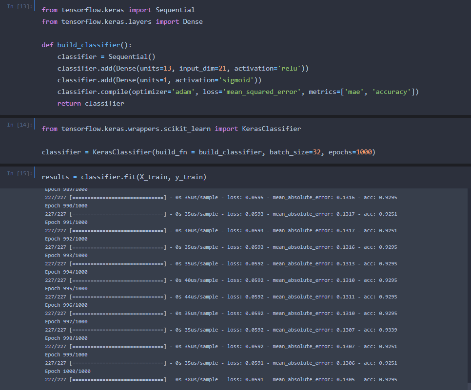
This code sets up a neural network with 14 hidden layers that iterate over the data 1000 times before determining a model configuration. Using “data science magic”, it passes the data through those hidden layers and activation functions, greatly increasing the accuracy of the model.
Deep Learning (Neural Network) Accuracy: 93.8%
Unfortunately, this is where most of the projects that I’ve seen online stop in regards to this database. People produce a model and say “Here’s my algorithm and it works”. For some reason, this really bothered me, as Machine Learning and Deep Learning are inherently useless without real world application, in my opinion. So we built this model. So what? What can the model be used for? How can new data be passed in? How can a doctor use this to speed up their practice, not waste time, and ultimately save their patient money?
Well, new data would need to be passed into the model and then the model would need to classify it based on what it’s learned before. Sounds simple enough in theory, but the application is tedious for multiple reasons.
But I did it anyway.
Deep Learning Program

Using Python, I wrote a program that will take user input for each variable, run it through the Deep Learning algorithm, and tell the user the presence of heart disease with an accuracy of 94%.
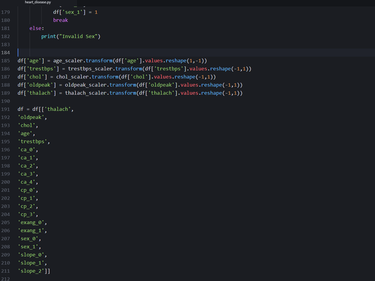
One of the problems is getting the variables to look exactly as they did when the algorithm was trained, including having OneHotEncoding and being scaled with the same MinMaxScalers. So, all of the scalers that were saved before were then imported back in and used on their respective fields. Meanwhile, the OneHotEncoding was built by hand. For much larger datasets, this would not be practical, but for this it was manageable.
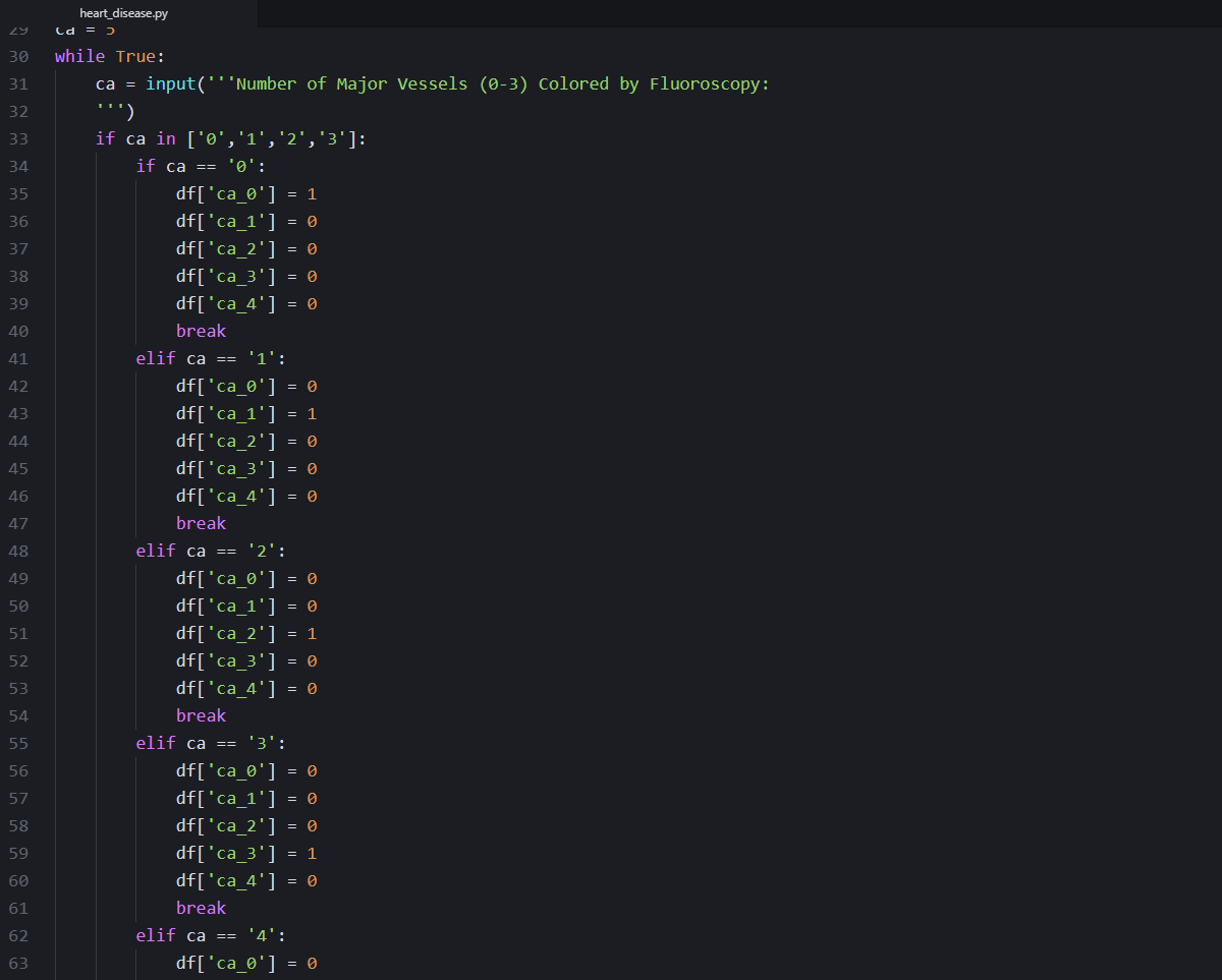
Once the program is run in command prompt or terminal, the user inputs data, and the program determines if the patient has heart disease or not.

Summary
This has a very real application in the real world, and could further be expounded upon by others in the data community. A user-friendly GUI and application could be made around the backend Python script, enabling doctors to screen their patients before more tests are needed. Eventually, as more data is collected, the model could get smarter and more accurate, allowing for even greater applications in the medical community. For now, with an accuracy of 94%, this tool could be used for screening and non-diagnostic purposes only, as even a 6% chance of a misdiagnosis is too large for someone to potentially be left untreated.